부록

‘R과 통계분석’ 연습문제 해답

“R과 통계분석” 3판에 있는 연습문제 중 일부 문제의 해답을 정리해서 보여드립니다.

2장

x <- c(17, 16, 20, 24, 22, 15, 21, 18)
x[length(x)]
## [1] 18

grade <- c("1st", "1st", "2nd", "3rd", "2nd", "3rd", "1st")
factor(grade)
## [1] 1st 1st 2nd 3rd 2nd 3rd 1st
## Levels: 1st 2nd 3rd

factor(grade, order = TRUE, level = c("3rd", "2nd", "1st"))
## [1] 1st 1st 2nd 3rd 2nd 3rd 1st
## Levels: 3rd < 2nd < 1st

x1 <- c(12, 17, 19)
x2 <- c(21, 22, 25)
x3 <- c(32, 34, 35)
d1 <- data.frame(var1 = x1, var2 = x2, var3 = x3)
d1
##   var1 var2 var3
## 1   12   21   32
## 2   17   22   34
## 3   19   25   35

d1["var2"]
##   var2
## 1   21
## 2   22
## 3   25

library(tidyverse)
df1 <- tibble(
  x = 1,
  y = 1:9,
  z = rep(1:3, each = 3),
  w=sample(letters, 9)
)

df1
## # A tibble: 9 × 4
##       x     y     z w    
##   <dbl> <int> <int> <chr>
## 1     1     1     1 x    
## 2     1     2     1 h    
## 3     1     3     1 p    
## 4     1     4     2 n    
## 5     1     5     2 d    
## 6     1     6     2 m    
## 7     1     7     3 j    
## 8     1     8     3 q    
## 9     1     9     3 c

df1[["y"]]
## [1] 1 2 3 4 5 6 7 8 9

df1[[2]]
## [1] 1 2 3 4 5 6 7 8 9

df1$y
## [1] 1 2 3 4 5 6 7 8 9

df1[1:5, 2]
## # A tibble: 5 × 1
##       y
##   <int>
## 1     1
## 2     2
## 3     3
## 4     4
## 5     5

as.data.frame(df1)[1:5, 2]
## [1] 1 2 3 4 5

a1 <- paste0(letters, 1:length(letters))
a1
##  [1] "a1"  "b2"  "c3"  "d4"  "e5"  "f6"  "g7"  "h8"  "i9"  "j10" "k11" "l12"
## [13] "m13" "n14" "o15" "p16" "q17" "r18" "s19" "t20" "u21" "v22" "w23" "x24"
## [25] "y25" "z26"

a2 <- paste(a1, collapse = "-")
a2
## [1] "a1-b2-c3-d4-e5-f6-g7-h8-i9-j10-k11-l12-m13-n14-o15-p16-q17-r18-s19-t20-u21-v22-w23-x24-y25-z26"

a3 <- gsub("-", "", a2)
a3
## [1] "a1b2c3d4e5f6g7h8i9j10k11l12m13n14o15p16q17r18s19t20u21v22w23x24y25z26"

y <- c(17, 16, 20, 24, 22, 15, 21, 18)

y[y == max(y)] <- 23                         
y
## [1] 17 16 20 23 22 15 21 18

sum(y >= 20)         
## [1] 4

mean(y <= 18)
## [1] 0.5

x <- c(1, 3, 2, 7, 12, 6, 1, 3, 6, 6, 7)
Y <- c(6.1, 9.7, 10.3, 18.8, 28.3, 16.1, 5.7, 12.6, 16.1, 15.8, 18.8)
X <- cbind(1,x)
beta.hat <- solve(t(X) %*% X)%*%t(X)%*%Y
rownames(beta.hat) <- c("beta_0", "beta_1")
colnames(beta.hat) <- c("Estimate")

beta.hat
##        Estimate
## beta_0 4.790317
## beta_1 1.955676

3장

library(rvest)
URL <- "https://en.wikipedia.org/wiki/South_Korea"
Xpath <- '//*[@id="mw-content-text"]/div[1]/table[7]'  # 2024.1.22 시점

tbl_1 <- read_html(URL) |>      # ' |> ' : pipe 연산자. 4장에서 소개됨. 
  html_nodes(xpath=Xpath) |> 
  html_table()

top_company <- tbl_1[[1]] 
names(top_company) <- c("Rank", "Name", "HQ", "Revenue", "Profit", "Assets")

print(top_company, n = 3)
## # A tibble: 15 × 6
##    Rank Name                HQ    Revenue Profit Assets 
##   <dbl> <chr>               <chr> <chr>   <chr>  <chr>  
## 1     1 Samsung Electronics Suwon 173,957 19,316 217,104
## 2     2 Hyundai Motor       Seoul 80,701  4,659  148,092
## 3     3 SK Holdings         Seoul 72,579  659    85.332 
## # ℹ 12 more rows

4장

library(tidyverse)

air_sub1 <- as_tibble(airquality) |>
  filter(Wind >= mean(Wind), Temp < mean(Temp)) |>
  select(Ozone, Solar.R, Month)

air_sub2 <- as_tibble(airquality) |>
  filter(Wind < mean(Wind), Temp >= mean(Temp)) |>
  select(Ozone, Solar.R, Month)

air_sub1 |> 
  summarize(n = n(), m_oz = mean(Ozone, na.rm = TRUE), 
            m_solar = mean(Solar.R, na.rm = TRUE))
## # A tibble: 1 × 3
##       n  m_oz m_solar
##   <int> <dbl>   <dbl>
## 1    42  17.6    166.

air_sub2 |> 
  summarize(n = n(), m_oz = mean(Ozone, na.rm = TRUE), 
            m_solar = mean(Solar.R, na.rm = TRUE))
## # A tibble: 1 × 3
##       n  m_oz m_solar
##   <int> <dbl>   <dbl>
## 1    55  71.4    204.

air_sub1 |>
  group_by(Month) |>
  summarize(n = n(), m_oz = mean(Ozone, na.rm = TRUE), 
            m_solar = mean(Solar.R, na.rm = TRUE))
## # A tibble: 5 × 4
##   Month     n  m_oz m_solar
##   <int> <int> <dbl>   <dbl>
## 1     5    17  19.1    181.
## 2     6     7  20.8    150.
## 3     7     1  10      264 
## 4     8     4  17.3    155.
## 5     9    13  15.6    152.

air_sub2 |>
  group_by(Month) |>
  summarize(n = n(), m_oz = mean(Ozone, na.rm = TRUE), 
            m_solar = mean(Solar.R, na.rm = TRUE))
## # A tibble: 5 × 4
##   Month     n  m_oz m_solar
##   <int> <int> <dbl>   <dbl>
## 1     5     1 115      223 
## 2     6     9  26      195 
## 3     7    20  71.5    232 
## 4     8    18  77.4    182.
## 5     9     7  63.9    181.

n <- 10
m <- 5
air <- airquality |> 
  slice_sample(n = n + m)
air_1 <- slice_head(air, n = n); air_1
##    Ozone Solar.R Wind Temp Month Day
## 1     NA     127  8.0   78     6  26
## 2      9      24 10.9   71     9  14
## 3     30     193  6.9   70     9  26
## 4     NA      98 11.5   80     6  28
## 5     NA     150  6.3   77     6  21
## 6     NA     242 16.1   67     6   3
## 7      9      24 13.8   81     8   2
## 8     35     274 10.3   82     7  17
## 9     NA     250  6.3   76     6  24
## 10    28      NA 14.9   66     5   6

air_2 <- slice_tail(air, n = m); air_2
##   Ozone Solar.R Wind Temp Month Day
## 1    NA     135  8.0   75     6  25
## 2    52      82 12.0   86     7  27
## 3    NA      91  4.6   76     6  23
## 4    31     244 10.9   78     8  19
## 5    NA     137 11.5   86     8  11

# 6장에서 소개되는 함수 anti_join()을 사용하는 방법
n <- 10
m <- 5
air_1 <- airquality |> 
  slice_sample(n = n); air_1
##    Ozone Solar.R Wind Temp Month Day
## 1     23     220 10.3   78     9   8
## 2     77     276  5.1   88     7   7
## 3     49     248  9.2   85     7   2
## 4     NA     135  8.0   75     6  25
## 5     NA     266 14.9   58     5  26
## 6      8      19 20.1   61     5   9
## 7     36     139 10.3   81     9  23
## 8     37     279  7.4   76     5  31
## 9    135     269  4.1   84     7   1
## 10    65     157  9.7   80     8  14

air_2 <- airquality |> 
  anti_join(air_1) |> 
  slice_sample(n = m); air_2
##   Ozone Solar.R Wind Temp Month Day
## 1    NA     194  8.6   69     5  10
## 2   108     223  8.0   85     7  25
## 3   115     223  5.7   79     5  30
## 4    44     236 14.9   81     9  11
## 5    78     197  5.1   92     9   2

car <- as_tibble(MASS::Cars93) |> 
  select(1:2, MPG.highway, Cylinders, Weight, Origin) |> 
  print(n = 3)
## # A tibble: 93 × 6
##   Manufacturer Model   MPG.highway Cylinders Weight Origin 
##   <fct>        <fct>         <int> <fct>      <int> <fct>  
## 1 Acura        Integra          31 4           2705 non-USA
## 2 Acura        Legend           25 6           3560 non-USA
## 3 Audi         90               26 6           3375 non-USA
## # ℹ 90 more rows

car <- car |> 
  mutate(make = paste(Manufacturer, Model), .before = 1) |> 
  select(!c(Manufacturer, Model)) |> 
  print(n = 3)
## # A tibble: 93 × 5
##   make          MPG.highway Cylinders Weight Origin 
##   <chr>               <int> <fct>      <int> <fct>  
## 1 Acura Integra          31 4           2705 non-USA
## 2 Acura Legend           25 6           3560 non-USA
## 3 Audi 90                26 6           3375 non-USA
## # ℹ 90 more rows

car |> count(Cylinders, sort = TRUE)
## # A tibble: 6 × 2
##   Cylinders     n
##   <fct>     <int>
## 1 4            49
## 2 6            31
## 3 8             7
## 4 3             3
## 5 5             2
## 6 rotary        1

car <- car |> 
  filter(Cylinders %in% c(4,6,8))

car |> 
  slice_max(MPG.highway, n = 2) |> 
  select(make, MPG.highway) 
## # A tibble: 2 × 2
##   make           MPG.highway
##   <chr>                <int>
## 1 Honda Civic             46
## 2 Pontiac LeMans          41

5장

data(barley, package = "lattice")

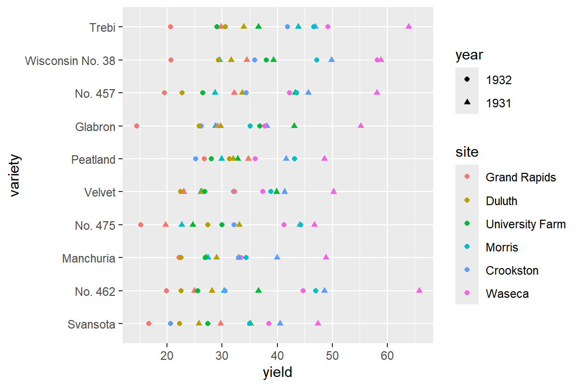
barley |>
  ggplot(aes(x = yield, y = variety, color = year)) +
  geom_point() +
  facet_wrap(facets = vars(site))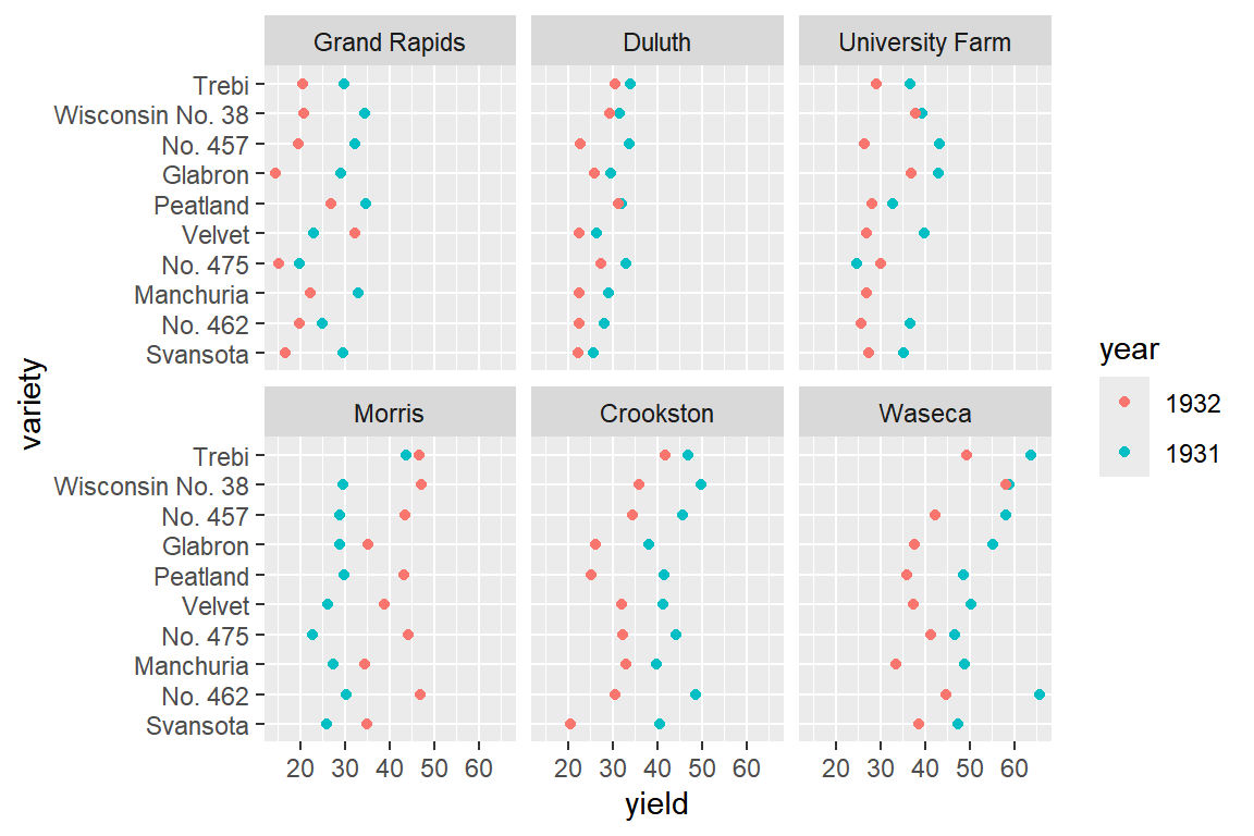

barley |>
  ggplot(aes(x = yield, y = variety, color = site, shape = year)) +
  geom_point()

barley |>
  group_by(variety) |>
  summarise(mean_yield = mean(yield)) |>
  arrange(desc(mean_yield))
## # A tibble: 10 × 2
##    variety          mean_yield
##    <fct>                 <dbl>
##  1 Trebi                  39.4
##  2 Wisconsin No. 38       39.4
##  3 No. 457                35.8
##  4 No. 462                35.4
##  5 Peatland               34.2
##  6 Glabron                33.3
##  7 Velvet                 33.1
##  8 No. 475                31.8
##  9 Manchuria              31.5
## 10 Svansota               30.4

airs <- as_tibble(airquality)

airs |>
  mutate(Missing = is.na(Ozone)) |>
  ggplot(aes(x = Month, fill = Missing)) +
  geom_bar(position = "fill") +
  labs(y = "Proportion of missing data")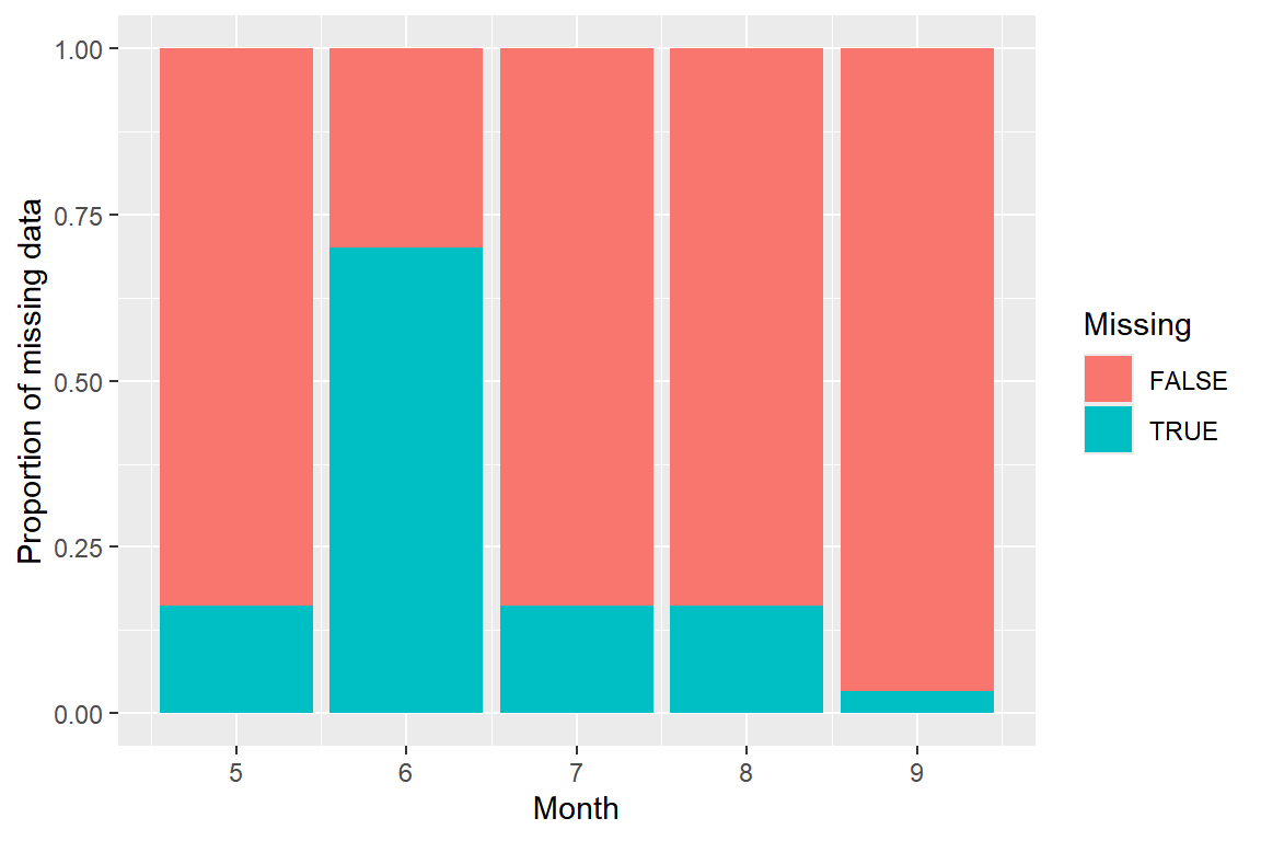 

airs |>
  group_by(Month) |>
  summarise(m.Oz = mean(Ozone, na.rm = TRUE)) |>
  ggplot(aes(x = Month, y = m.Oz)) +
  geom_bar(stat = "identity", fill = "steelblue") +
  labs(y = "Mean Ozone")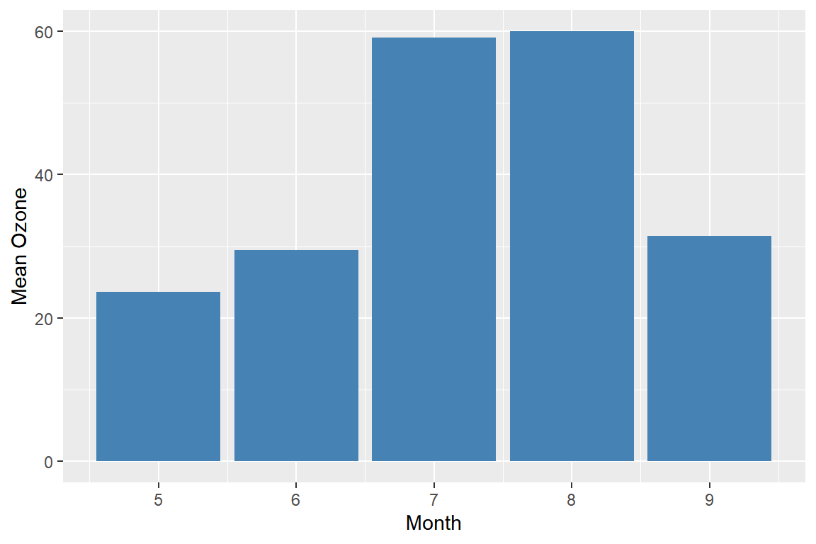

airs |>
  mutate(gp_Wind = if_else(Wind >= mean(Wind), 
                         "High Wind","Low Wind"),
         gp_Temp = if_else(Temp >= mean(Temp), 
                         "High Temp","Low Temp")) |>
  ggplot(aes(x = Solar.R, y = Ozone)) +
  geom_point() +
  facet_grid(rows = vars(gp_Wind), cols = vars(gp_Temp))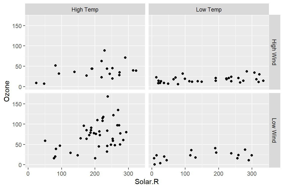 

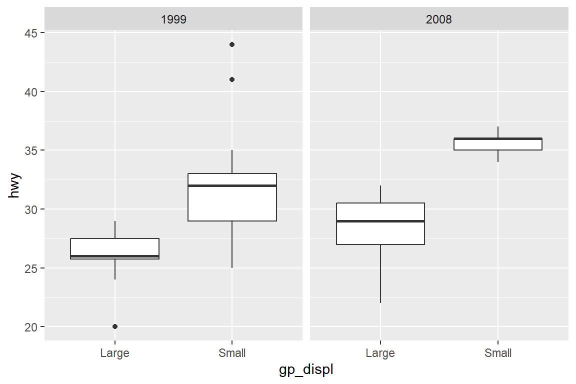
mpg_1 <- mpg |>
  filter(cyl == 4) |>
  mutate(year = factor(year)) |>
  select(model, year, displ, cty, hwy) |>
  arrange(year, desc(displ), cty) |>
  print(n = 5)
## # A tibble: 81 × 5
##   model             year  displ   cty   hwy
##   <chr>             <fct> <dbl> <int> <int>
## 1 4runner 4wd       1999    2.7    15    20
## 2 toyota tacoma 4wd 1999    2.7    15    20
## 3 4runner 4wd       1999    2.7    16    20
## 4 toyota tacoma 4wd 1999    2.7    16    20
## 5 forester awd      1999    2.5    18    25
## # ℹ 76 more rows

p2 <- mpg_1 |> 
  mutate(gp_displ = if_else(displ >= 2.0, "Large","Small")) |>
  ggplot()

p2 + 
  geom_jitter(aes(x = cty, y = hwy, color = gp_displ), size = 2) +
  facet_wrap(vars(year), ncol = 1) +
  labs(color = "Displacement \nGroup")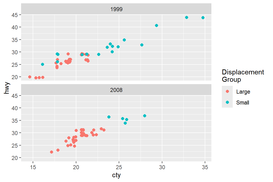

p2 + 
  geom_boxplot(aes(x = gp_displ, y = hwy)) +
  facet_wrap(vars(year)) 

6장

top_100 <- billboard |>  
  pivot_longer(
    cols = starts_with("wk"),
    names_to = "week",
    names_prefix = "wk",
    names_transform = list(week = as.integer),
    values_to = "rank",
    values_drop_na = TRUE
    ) |> 
  print(n = 10)
## # A tibble: 5,307 × 5
##    artist  track                   date.entered  week  rank
##    <chr>   <chr>                   <date>       <int> <dbl>
##  1 2 Pac   Baby Don't Cry (Keep... 2000-02-26       1    87
##  2 2 Pac   Baby Don't Cry (Keep... 2000-02-26       2    82
##  3 2 Pac   Baby Don't Cry (Keep... 2000-02-26       3    72
##  4 2 Pac   Baby Don't Cry (Keep... 2000-02-26       4    77
##  5 2 Pac   Baby Don't Cry (Keep... 2000-02-26       5    87
##  6 2 Pac   Baby Don't Cry (Keep... 2000-02-26       6    94
##  7 2 Pac   Baby Don't Cry (Keep... 2000-02-26       7    99
##  8 2Ge+her The Hardest Part Of ... 2000-09-02       1    91
##  9 2Ge+her The Hardest Part Of ... 2000-09-02       2    87
## 10 2Ge+her The Hardest Part Of ... 2000-09-02       3    92
## # ℹ 5,297 more rows

다른 방법

top_100 <- billboard |> 
  pivot_longer(cols = starts_with("wk"),
               names_to = "week",
               values_to = "rank"
               ) |> 
  mutate(week = parse_number(week)) |> 
  drop_na(rank) |> 
  print(n = 10)
## # A tibble: 5,307 × 5
##    artist  track                   date.entered  week  rank
##    <chr>   <chr>                   <date>       <dbl> <dbl>
##  1 2 Pac   Baby Don't Cry (Keep... 2000-02-26       1    87
##  2 2 Pac   Baby Don't Cry (Keep... 2000-02-26       2    82
##  3 2 Pac   Baby Don't Cry (Keep... 2000-02-26       3    72
##  4 2 Pac   Baby Don't Cry (Keep... 2000-02-26       4    77
##  5 2 Pac   Baby Don't Cry (Keep... 2000-02-26       5    87
##  6 2 Pac   Baby Don't Cry (Keep... 2000-02-26       6    94
##  7 2 Pac   Baby Don't Cry (Keep... 2000-02-26       7    99
##  8 2Ge+her The Hardest Part Of ... 2000-09-02       1    91
##  9 2Ge+her The Hardest Part Of ... 2000-09-02       2    87
## 10 2Ge+her The Hardest Part Of ... 2000-09-02       3    92
## # ℹ 5,297 more rows

top_100 |>  
  filter(rank == 1) |> 
  group_by(artist, track) |> 
  filter((max(week) - min(week) + 1) == n()) |> 
  count(sort = TRUE) |> 
  print(n=2)
## # A tibble: 16 × 3
## # Groups:   artist, track [16]
##   artist          track                       n
##   <chr>           <chr>                   <int>
## 1 Destiny's Child Independent Women Pa...    11
## 2 Santana         Maria, Maria               10
## # ℹ 14 more rows

part_df <- tibble(num = c(155, 501, 244, 796),
                  tool = c("screwdrive", "pliers", "wrench", "hammer"))
order_df <- tibble(num = c(155, 796, 155, 244, 244, 796, 244),
                   name = c("Park", "Fox", "Smith", "White", "Crus", "White", "Lee"))

part_df |> left_join(order_df, by = join_by(num))
## # A tibble: 8 × 3
##     num tool       name 
##   <dbl> <chr>      <chr>
## 1   155 screwdrive Park 
## 2   155 screwdrive Smith
## 3   501 pliers     <NA> 
## 4   244 wrench     White
## 5   244 wrench     Crus 
## 6   244 wrench     Lee  
## 7   796 hammer     Fox  
## 8   796 hammer     White

part_df |> inner_join(order_df, by = join_by(num))
## # A tibble: 7 × 3
##     num tool       name 
##   <dbl> <chr>      <chr>
## 1   155 screwdrive Park 
## 2   155 screwdrive Smith
## 3   244 wrench     White
## 4   244 wrench     Crus 
## 5   244 wrench     Lee  
## 6   796 hammer     Fox  
## 7   796 hammer     White

str_c(letters, LETTERS, collapse = "")
## [1] "aAbBcCdDeEfFgGhHiIjJkKlLmMnNoOpPqQrRsStTuUvVwWxXyYzZ"

7장

res <- vector("double", 12)
res[1] <- 0; res[2] <- 1
for(i in 1:10){
  res[i+2] <- res[i]+res[i+1]
}
res
##  [1]  0  1  1  2  3  5  8 13 21 34 55 89

airs_M <- airquality |> 
  select(-c(Month, Day)) |>
  split(airquality$Month)

map(airs_M, ~map_dbl(.x, mean, na.rm = TRUE))
## $`5`
##     Ozone   Solar.R      Wind      Temp 
##  23.61538 181.29630  11.62258  65.54839 
## 
## $`6`
##     Ozone   Solar.R      Wind      Temp 
##  29.44444 190.16667  10.26667  79.10000 
## 
## $`7`
##      Ozone    Solar.R       Wind       Temp 
##  59.115385 216.483871   8.941935  83.903226 
## 
## $`8`
##      Ozone    Solar.R       Wind       Temp 
##  59.961538 171.857143   8.793548  83.967742 
## 
## $`9`
##     Ozone   Solar.R      Wind      Temp 
##  31.44828 167.43333  10.18000  76.90000

map(airs_M, ~map_dbl(.x, ~sum(is.na(.x))))
## $`5`
##   Ozone Solar.R    Wind    Temp 
##       5       4       0       0 
## 
## $`6`
##   Ozone Solar.R    Wind    Temp 
##      21       0       0       0 
## 
## $`7`
##   Ozone Solar.R    Wind    Temp 
##       5       0       0       0 
## 
## $`8`
##   Ozone Solar.R    Wind    Temp 
##       5       3       0       0 
## 
## $`9`
##   Ozone Solar.R    Wind    Temp 
##       1       0       0       0

airquality |>
  group_by(Month) |>
  summarise(across(1:4, list(Mean = ~mean(.x, na.rm = TRUE))))
## # A tibble: 5 × 5
##   Month Ozone_Mean Solar.R_Mean Wind_Mean Temp_Mean
##   <int>      <dbl>        <dbl>     <dbl>     <dbl>
## 1     5       23.6         181.     11.6       65.5
## 2     6       29.4         190.     10.3       79.1
## 3     7       59.1         216.      8.94      83.9
## 4     8       60.0         172.      8.79      84.0
## 5     9       31.4         167.     10.2       76.9

airquality |>
  group_by(Month) |> 
  summarise(across(1:4, list(miss = ~sum(is.na(.x)))))
## # A tibble: 5 × 5
##   Month Ozone_miss Solar.R_miss Wind_miss Temp_miss
##   <int>      <int>        <int>     <int>     <int>
## 1     5          5            4         0         0
## 2     6         21            0         0         0
## 3     7          5            0         0         0
## 4     8          5            3         0         0
## 5     9          1            0         0         0

참고문헌

Becker, Chambers, R. A., and A. R. Wilks. 1988. The New s Language: A Programming Environment for Data Analysis and Graphics. Pacific Grove, California: Wadsworth & Brooks/Cole Advanced Books & Software.

Cleveland, William S. 1993. Visualizing Data. New Jersey: Hobart Press.

Jones, Mailardet, O., and A Robinson. 2009. Introduction to Scientific Programming and Simulation Using r. Chapman & Hall/CRC.

Venables, W. N., and B. D. Ripley. 2000. S Programming. Springer-Verlag.

Wickham, Hadley. 2019. Advanced r. 2nd ed. CRC Press.